Last year at the first Clojure Conj, for some reason or another I started pondering ways to improve on the classic lazy-list-of-primes (which I took a quasi stab at in an old post). Most of the simpler examples use division to check primality, which performs terribly compared to addition-based algorithms like the Sieve of Eratosthenes.
However, sieve implementations usually compute huge chunks of primes at once, while I wanted to be able to compute one prime at a time, hopefully using Clojure’s iterate function. I wanted it to perform similarly to the classic sieve in terms of time, and to have space requirements proportional to the square root of the prime being computed (particularly not holding the entire preceding sequence of primes in memory when only a fraction of that is actually needed).
So after thinking about the structure of the sieve algorithm for a bit, I realized that it actually was amenable to computing primes iteratively. In the classic sieve algorithm, given a candidate range, for each relevant small prime you sweep through the range marking off the multiples of that prime. The prime numbers in the range are those that remain after all the small primes have swept through. The key to making this iterative is, given a prime, rather than sweeping through an array, you just keep track of its next multiple. When that multiple comes up as a candidate, you mark it as composite, and then update your “next multiple” value for that prime. Of course you have to juggle several small primes instead of just one, so this might be a good point to bring up the actual code.
We start with the following object:
(def initial
  {:p        3,
   :divisors {9 '(3)},
   :square   9,
   :primes   nil})
The value of :p is the current prime. We first create a lazy seq of objects like this one, and turning that into a seq of primes is simply mapping to the value of :p. The value of :divisors is the data structure partially described in the previous paragraph. It is a map whose keys are upcoming composite numbers, and whose values are the primes relevant to those composites. The first odd composite to be on the lookout for is 9, and the only prime corresponding to it is 3. The last two keys, :square and :primes, are used for adding primes to the :divisors map. The value of :square tells us when to add a new prime, and the value of :primes will tell us what that prime is.
Let’s see how the initial object is iterated. The initial object corresponds to the prime 3, so the next object corresponds to the prime 5:
{:p        5,
 :divisors {9 (3)},
 :square   9,
 :primes   nil}
Not much changed. The only difference is that :p now maps to 5 instead of 3. This will also be the case for 7, so let’s skip that and go right to 11:
{:p        11,
 :divisors {15 (3), 25 (5)},
 :square   25,
 :primes   {:p 5, :divisors {9 (3)}, :square 9, :primes nil}}
There’s been a few changes here. When the 7 object was passed to the iterator function, it incremented 7 to 9 and checked if 9 was present in the :divisors map. Since it was, it knew that 9 was composite. First it updated the :divisors map from {9 (3)} to {15 (3)}, by computing that the next composite for three is 9 + 3 * 2 (we double the prime since we’re skipping even numbers). Then it checked if the current number under consideration (9) was equal to the value of :square. Since it was, it computed the next prime to add to the :divisors hash, which is of course 5. Computing the next prime, however, requires a bit of recursion, since computing primes is the actual task at hand. So the :primes key ends up pointing to a nested version of the exact object we’re looking at, and if you look at the :primes object above you can see it’s identical to the entire object given for p = 5.
This recursion is how we avoid keeping the entire list of primes in memory. Let’s see what the object looks like after computing the 10000th prime:
{:p 104729,
 :divisors
   {104737 (17 61 101),
    104833 (79),
    104993 (283),
    104835 (241),
    104867 (71 211),
    104931 (131),
    105187 (293),
    104741 (7 13),
    104805 (137),
    104775 (127),
    104807 (311),
    104777 (29),
    104809 (163),
    104873 (199),
    104937 (263),
    105001 (197),
    105033 (157 223),
    104747 (19 37 149),
    104843 (59),
    104749 (31 109),
    104781 (53),
    104813 (281),
    104877 (271),
    105101 (227),
    104751 (103 113),
    104753 (89 107),
    104945 (139 151),
    105073 (179),
    105169 (251),
    104755 (41 73),
    105011 (173),
    105043 (167),
    105301 (307),
    104791 (43),
    104855 (67 313),
    104983 (277),
    105111 (229),
    104857 (97),
    104921 (239),
    105113 (257),
    109561 (331),
    104731 (11),
    104763 (47),
    104859 (191),
    105083 (233),
    105179 (269),
    104733 (3),
    104765 (23),
    104829 (83),
    104735 (5),
    104799 (181 193),
    104927 (317)},
 :square 109561,
 :primes
   {:p 331,
    :divisors
      {343 (7), 333 (3), 351 (13), 335 (5), 357 (17), 341 (11), 361 (19)},
    :square 361,
    :primes
      {:p 19,
       :divisors {21 (3), 25 (5)},
       :square 25,
       :primes {:p 5, :divisors {9 (3)}, :square 9, :primes nil}}}}
As you can see there are several layers of nesting going on. This nesting does not create much performance overhead, since the nested versions don’t get very far relative to the main sequence, and I think it makes the algorithm simpler.
I did some minor googling to see if anybody else had done something like this, and I did find one that was quite similar. However, it looks like that programmer used explicit nested lazy seqs, while I wanted to keep the nested seqs implicit so the the objects iterated over remained finite.
Anyhow, here’s the full source code. I have a difficult time explaining algorithms like this clearly, so I will consider myself lucky if I’ve successfully communicated to a single person.
Bags and Trees
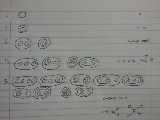
2011-04-05Was doodling in class recently:
And so of course this led to the discovery of Sloane A000081. For some reason I wasn’t expecting the rooted trees connection (I didn’t draw them until after I had read about it).
Comments
Periodic Curved Sequences
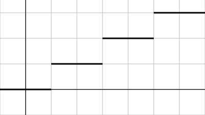
2011-03-03Given a sequence of integers, a common mathematical task is to try to find a short “closed” form for the sequence. For example, a closed form for (2,6,12,20,…) is n*(n+1), a closed form for (-1,1,-1,1,-1,…) is (-1)^n, and a closed form for (1,1,2,2,3,3,…) is floor((n+1)/2) (where the floor function rounds down).
The last two are interesting because they are not continuous. This means that if you interpreted the ‘closed form’ as a function of real numbers and plotted it on a graph, you would not see a smooth continuous line. In the case of floor((n+1)/2), you would see horizontal lines each two units long, and each one one unit higher than the previous:
In the case of (-1)^n, I don’t think there’s any kind of continuity whatsoever. You might be able to say that the function is defined when n is rational, but I think that’s as far as it goes.
For some reason that I can’t properly justify, I don’t like this. I like it when an integer sequence can be generated by a continuous smooth curve. Any finite sequence can be generated by a polynomial with a degree that is at most one less than the length of the sequence, which is exactly what my sequences-to-functions app does. For example, the sequence (1,2,3,4,1) can be generated by the polynomial (-1/6)x^4 + (5/3)x^3 – (35/6)x^2 + (28/3)x – 4:
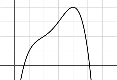
Of course, the next value generated by the polynomial is not 2, as the sequence suggests, but -14. In general any polynomial generated by a sequence like this will rocket upward or downward at either end. So you can’t get any kind of periodic behavior out of polynomials. I started investigating using the sine function for periodic behavior back in high school when I first encountered the double-counting sequence (1,1,2,2,3,3,…).
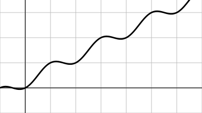
The sine curve can help when we note that the double counting sequence can be written as the sum of two other simpler sequences:
   0.5,  1.0,  1.5,  2.0,  2.5,  3.0,  3.5,  4.0,  ...
 + 0.5,  0.0,  0.5,  0.0,  0.5,  0.0,  0.5,  0.0,  ...
-------------------------------------------------------
   1.0,  1.0,  2.0,  2.0,  3.0,  3.0,  4.0,  4.0,  ...
The first of these is simply f(x) = x/2, and the second is a simple alternation between 0 and 0.5. The sine curve is great at alternating, so all we need is to stretch and pull it to make everything line up correctly:
This was as far as I thought about the issue in high school, and aside from a brief resurfacing in college calculus, it didn’t come to mind again until recently when a friend of mine started taking calculus. Only then did I realize that there are glaring questions here: What other sequences can we produce with these tools? What periods can they have? Would anybody like a beer?
So I’ve thought about these questions some during my spare moments the last few weeks, and have a few answers so far. The first thing I noted was that, for a given period, there is a canonical sequence that we may as well call a “basis”, from which any periodic sequence can be constructed. The simplest for a period P is simply P-1 zeros followed by a single one. For example, with P = 5, the canonical sequence (call it ‘the 5-basis’) would be (0,0,0,0,1,0,0,0,0,1,0,…). This is sufficient to create any period-5 sequence by simply shifting back and forth and multiplying. If our canonical sequence is called f(n), and we want to create the sequence (1,9,6,2,5,1,9,6,2,5,1,…), we can do each of the five numbers individually and then add them together:
g(n) = f(n+4) + 9*f(n+3) + 6*f(n+2) + 2*f(n+1) + 5*f(n)

   1, 0, 0, 0, 0, 1, 0, 0, 0, 0, 1, ...
   0, 9, 0, 0, 0, 0, 9, 0, 0, 0, 0, ...
   0, 0, 6, 0, 0, 0, 0, 6, 0, 0, 0, ...
   0, 0, 0, 2, 0, 0, 0, 0, 2, 0, 0, ...
 + 0, 0, 0, 0, 5, 0, 0, 0, 0, 5, 0, ...
----------------------------------------
   1, 9, 6, 2, 5, 1, 9, 6, 2, 5, 1, ...
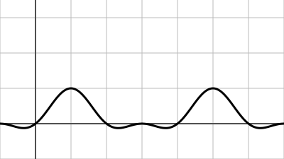
So finding a basis function gives us a lot. It also gives us the repeated counting function for its period (for period P, start with f(x) = x/P and then subtract off appropriate amounts using P-1 fractional multiples of the basis). The next question then is what basis functions can we construct from the sine function? The basis for P=2 is not hard, since the most obvious characteristic of the sine function is that it alternates between two values. P=4 also turns out to be pretty easy, because the sine function also has a clean period-4 version, which isn’t a basis function but can easily produce a basis function when combined with the 2-basis:
| f(n) = (1+sin(πn – 1/2))/2 | = 1, 0, 1, 0, 1, 0, 1, 0, 1, … |
| g(n) = sin(πn/2) | = 1, 0,-1, 0, 1, 0,-1, 0, 1, … |
| h(n) = (f(n) + g(n))/2 | = 1, 0, 0, 0, 1, 0, 0, 0, 1, … |
The 4-basis can be used to create a period-4 counting loop:
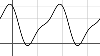
This was as far as I got at first — I wasn’t sure if I could use the sine function to create a basis for any periods other than 2 and 4. Eventually I weasled out a period-3 basis using a single sine wave:
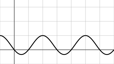
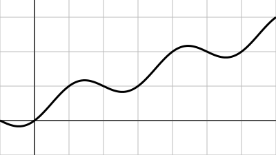
Which we can of course use to make a triple-counting function:
And most recently using all sorts of shameful tricks I found a basis for period-5:
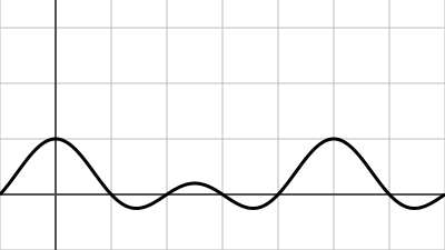
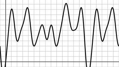
I haven’t yet figured out if the witchcraft that was involved can be used for higher prime periods, of if there is any hope for aperiodic sequences like (1,2,1,2,3,1,2,3,4,1,2,3,4,5,1,…). But I do know that if you multiply the 3-basis with the 5-basis you get a 15-basis, and so I have no choice but to conclude with a graph for a period-15 sequence of random integers from 0 to 10:
Comments
The Dvorak Permuation
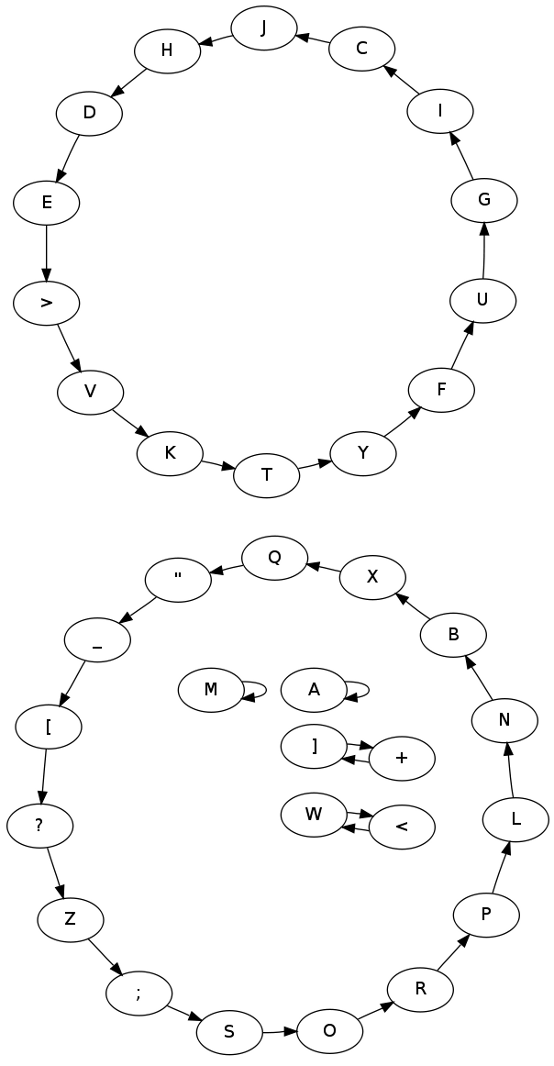
2011-02-28Apparently, the Qwerty-to-Dvorak keyboard permutation, which I just performed on an office keyboard, contains two large cycles, two double cycles (bicycles?), and two trivial cycles:
Comments
Two Thousand and Eleven
2011-01-03Easily convinced friends, your computer, and various internet sources not held accountable to any standard of accuracy may assert that 2011 is a prime number, but it would be foolish to blindly accept the claims of uninformed sheeple and agenda-driven pundits. If you’re interested in discovering the truth about this important issue and want to verify the primality yourself by hand, it should be sufficient to check the following equations:
2 × 1005 + 1 = 2011
3 × 670 + 1 = 2011
5 × 402 + 1 = 2011
7 × 287 + 2 = 2011
11 × 182 + 9 = 2011
13 × 154 + 9 = 2011
17 × 118 + 5 = 2011
19 × 105 + 16 = 2011
23 × 87 + 10 = 2011
29 × 69 + 10 = 2011
31 × 64 + 27 = 2011
37 × 54 + 13 = 2011
41 × 49 + 2 = 2011
43 × 46 + 33 = 2011
45 × 45 = 2025
Don’t immediately accept what you’re told! Always check the facts.
Comments