Spending some time on a treadmill got me thinking about the experience of tracking the passage of a fixed period of time. Sometimes people like to note numeric milestones, like when the period is halfway over. These numeric milestones can come in different flavors depending on whether you're thinking about percentages, or time units like days or minutes. But it occurred to me that the experience of noting these milestones can be more engaging when the milestones aren't uniformly spaced.
Due to my affinity for harmonic numbers, I would start noticing when I had finished 1/5 of the distance I was running, then 1/4, 1/3, and 1/2, and then for symmetry also 2/3, 3/4, 4/5, etc. This meant that the milestones were clustered around the beginning and end of the period, which was kind of interesting. But this had the downside that the time between the more central milestones could be rather long. Instead of breaking these up with other fractions like 3/5, it occurred to me that I could recursively track the spacing between milestones. For example, if I was waiting for the time period to progress from 1/2 to 2/3, but this progression would itself take a long time, I could notice when I'm halfway from 1/2 to 1/3, and then 2/3 of the way from 1/2 to 2/3, etc. This is obviously difficult to take very far using mental arithmetic, but I realized a computer could take it as far as you like. This means that very long time periods, of years or more, can be decomposed into non-uniform intervals such that there's always some kind of arguably-interesting milestone happening, and it's generally going to be somewhat different from the ones that have happened recently and the ones that will be happening shortly.
So I put together a thing that visualizes this for you, using a series of clock-like things:
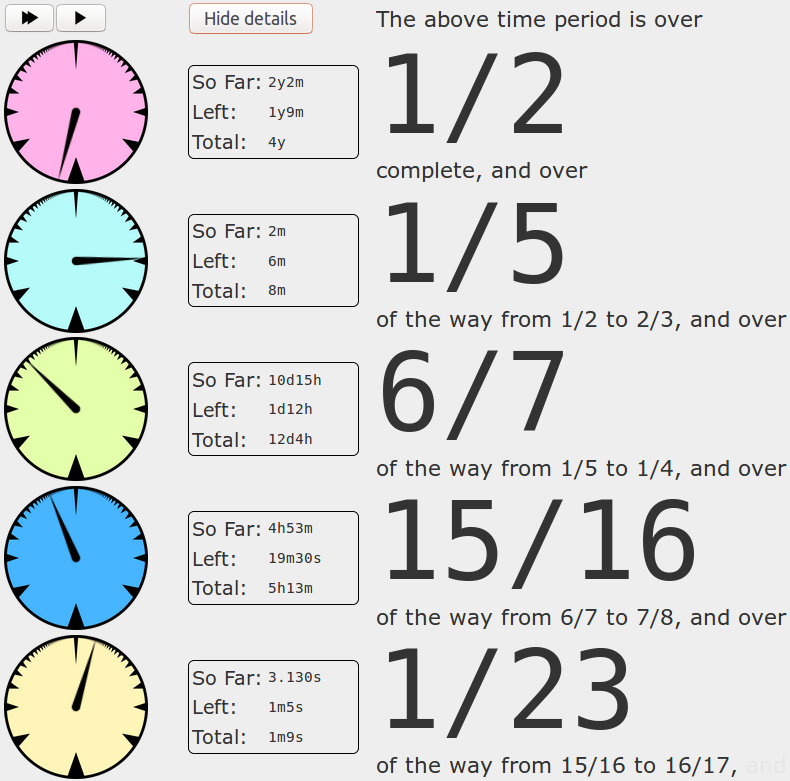
You can set it up with a specific time interval, or just start a new one from the current time. This is it right here.
Thanks to Carissa Miller and Tim Galeckas for valuable feedback.
A Polyomino Tiling Algorithm
2018-08-18UPDATE: Thanks to David MacIver for pointing out that the problem being reduced to here is the Exact Cover problem, and the reduction was described by Donald Knuth in his Dancing Links paper.
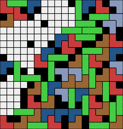
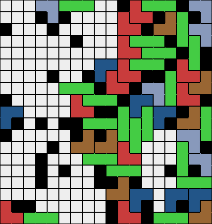
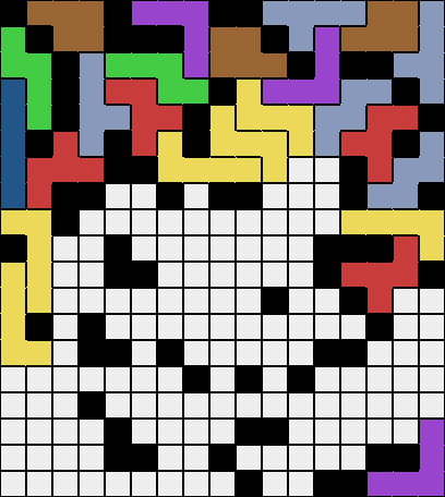
Over eight years ago I created the Polyomino Tiler (a browser application that attempts to tile arbitrary grids with sets of polyominoes), but I haven't ever written about the algorithm it uses.
If any aspects of what follows are confusing, it may help to play with the polyomino tiler a bit to get a better idea for what it's doing.
There are a couple aspects of the problem that combine to make it challenging:
- the set of available polyominos is fully customizable up to the heptominoes; each polyomino can be restricted to specific flips/rotations
- the grid can be any subset of a rectangular grid (or a cylinder/torus)
So the algorithm needs to be generic enough to not get bogged down in all the edge cases resulting from these two facts.
The two key components of the algorithm are:
- abstract away the geometric details by constructing a graph that describes all the possibilities
- apply certain heuristics to a generic backtracking search algorithm on that graph
Placements
The main preprocessing step is to calculate all possible placements of all available pieces. When hundreds of piece variants are available this step can be lengthy, and the result can require a lot of memory. But the result is essentially a bipartite graph (or, in database terms, a many-to-many relationship) between placements and grid points.
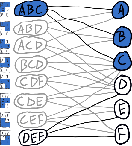
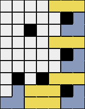
For example, given this 2x3 grid:
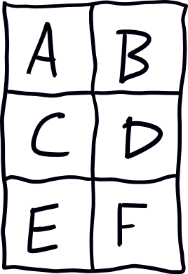
and restricting ourselves to the L-shaped trominoes to keep the visuals tractable, the placement graph looks like this:
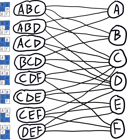
Notice that all of the geometric details have been abstracted away; this means that the rest of the algorithm could just as easily be applied to grids of triangles, or hexagons, or hyperbolic grids, or higher dimensions.
Search
Given the bipartite graph, the problem of tiling the grid can be reformulated as the problem of finding a subset of the placements that, as a whole, is connected to every one of the grid points exactly one time.
The search algorithm is a backtracking algorithm that at each step chooses an untiled grid point and a random placement associated with that grid point; it adds that placement to the solution set and then tries to tile the remainder of the grid (taking note of which placements are invalidated by the one selected). If it fails to tile the rest of the grid, then it tries the next placement. If it runs out of placements, then the grid must be untileable.
For example, if we decide to start tiling the above grid from grid point A, the search tree might look like this:
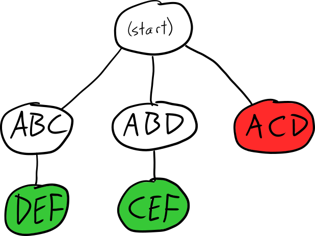
Depending on the order that we search the children, we could either end up with the ABC-DEF tiling or the ABD-CEF tiling; if we visit the ACD branch first, we'll have to backtrack since there's no solution in that direction.
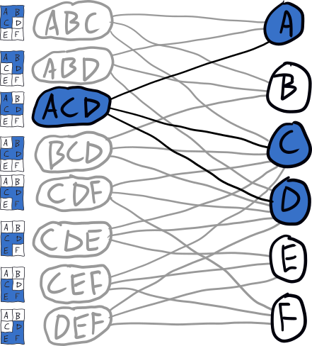
The reason the tree is so sparse is that each time we descend we remove placements from the graph that conflict with the one chosen. E.g., when we descend to ABC, the graph is updated to look like this:
This basic search algorithm is specialized with several heuristics/optimizations.
Untileability from Zero Placements
Since every placement we select makes several other placements impossible, it's easy to get to a point where there is some grid point that no longer has any possible placements. This is the most common sign of untileability, and it means we need to backtrack and try something different.
For example, if we descended down the ACD branch of the search tree, the graph would look like this, and the existence of grid points with no placements indicates that there's no solution.
Untileability with Number Theory
A given set of polyominoes places restrictions on what grids can be tiled purely based on their size. This is solely a function of the set of distinct sizes of the polyominoes.
For example, with the tetrominoes, only grids whose size is a multiple of four can be tiled. If the polyominoes have sizes 4 and 6, then only grids whose size is an even number greater than two can be tiled. This kind of analysis is closely related to the coin problem.
Further, if a grid consists of disconnected subcomponents, then we can analyze the tileability of each one separately, and conclude that the whole grid can't be tileable if any of the subcomponents is not tileable.
For example, this grid has been disconnected, and even though the size of both pieces together is a multiple of three and so could theoretically be tiled by trominoes, the individual subcomponents do not have a multiple of three grid points, and so neither of them are tileable.
Smallest Subcomponents First
If the grid at any point becomes disconnected, we immediately restrict the algorithm to the smallest subcomponent and try to tile that completely before moving on to the next one. The logic here is that if the disconnected grid as a whole can't be tiled, there's a decent chance that the smallest subcomponent can't be tiled. The smallest subcomponent is also likely the one that we can finish searching the fastest, and so this hopefully leads to a more aggressive pruning of the search space.
For example, this grid has a small component and a large component, and the small component can't be tiled with trominoes (can you figure out why?); tiling the smaller one first means we find out about this problem quickly, rather than waiting until the whole large subcomponent has been tiled.
Tile the most restricted grid points first
Within a subcomponent, we select the next grid point to tile based on the number of remaining placements it has. It is not uncommon for there to be a grid tile with only a single option, and in those cases it's important to place that piece immediately, since it likely decreases the size of the search space by eliminating other placements (and potentially causing more grid points to have only one option).
When there's not a grid point with a single placement, we still prioritize grid points with the fewest number of placements, since these are intuitively the most "difficult" parts of the grid to tile, which makes them more likely to be rendered untileable by other placements.
For example, in this grid the untiled grid point in the bottom left corner has only one possible placement with trominoes; tiling it lets us eliminate seven other placements that conflict with the forced placement.
Split the grid whenever possible
The last heuristic is a little crude but still useful. The motivation is that being able to split the grid into subcomponents is useful (since they can be analyzed independently), and so if we have the opportunity to split it by placing a piece, we should do so. So the precise rule is that, when there aren't any single-placement grid points (which are higher priority), and there is a single grid point that splits the grid (in graph theory terms, a vertex whose removal disconnects the graph), then we search placements for that grid point next.
For example, there are a couple grid points that disconnect the bottom right portion of this grid from the rest of it; either of these could be chosen for the next search step.
This approach could probably be generalized to something that tends to select grid points that make the grid easier to split, rather than only acting on this principle when it can be achieved in a single step. However, this would likely be somewhat in tension with the prioritization of the most restricted grid points, so I'm not sure how it would work out.
Getting Stuck
Since the polyomino tiling problem is NP-complete, it's not surprising that there's a variety of scenarios where the algorithm gets stuck. Some of these are artifacts of the particular algorithm, and it could conceivably be tweaked to handle those special cases. But I think the algorithm as it is is a decent balance of broad efficacy and simplicity.
The randomness in the algorithm (the ordering of placements for a particular grid point, and to a limited extent the prioritization of grid points) means that sometimes more progress can be made simply by restarting the search.
Possibilities
There are a variety of directions the algorithm could be tweaked; I mentioned one earlier about working more aggressively to split the grid.
Another idea is to optimize the order that placements for a particular grid point are tried. Perhaps placements could be prioritized based on the number of options available for the other grid points involved.
Summary
So to tile an arbitrary grid with an arbitrary set of polyominoes, we:
- calculate all possible placements to obtain a bipartite graph between grid points and placements
- use a backtracking algorithm to search for a subset of placements that exactly tiles the grid
- optimize the algorithm by using various heuristics to prioritize its choices
In hindsight, I believe the initial step of transforming to a graph could be retargeted to transforming to an instance of the SAT problem, in which case a generic SAT solver could be used for the rest of the algorithm. It would be interesting to learn which of the heuristics in my algorithm have analogs in general SAT solvers, and which are particular to tiling problems.
Comments
Visualizing Hash Functions
2013-06-03I've been working on some static visualizations of hash functions, starting with SHA1 and MD5 (images here and here, respectively). The two sample images show the process of computing the respective hash functions on the input "denny" (with ASCII encoding -- i.e., the input in hex is "64656E6E79"). A portion of the MD5 image is included below:

Notes about these two particular algorithms and their visualizations:
- Both algorithms are mostly defined in terms of operations on 32-bit "words", which essentially means 32-bit integers. They define the input/output conversion from sequences of bits/bytes to words, but this step is not covered in the diagrams.
- Probably the most confusing thing if you examine them in detail is that SHA1 uses a big-endian conversion from 4 bytes to 1 word while MD5 uses little-endian. See Appendix A for more. (tl;dr: the words in MD5 have their bytes printed in the opposite order you would expect.)
- MD5 and SHA1 have a lot of similarities, and in particular they both include a function of 3 words that varies slightly throughout the computation; so I've highlighted this function with a yellow box.
- The way that MD5 evolves its state is very similar to SHA1, but it is described differently in the spec. I decided to deviate from the spec and structure the diagram the same way as SHA1, which both highlights the similarity and is also (I think) a bit simpler to follow.
If you're curious about any other details of MD5 or SHA1, the specs are fairly readable, hopefully even more so with the diagrams to follow along with.
I'm hoping this sort of diagram can
- give an appreciation for
- how complex hash functions are, both absolutely and relative to each other
- the difficulty of trying to invert a cryptographic hash function
- be a useful aid to anyone trying to understand the details of a particular algorithm
- be fun to look at. I love things that give a sense for how crazy-complicated computers look from certain angles.
Several things I think are worth exploring:
- How well can this approach be adapted to hairier algorithms?
- Whirlpool uses a 64-byte state rather than a 5-word state (like SHA1)
- A more esoteric algorithm could operate on individual bits
- I'd like to branch out into other sorts of computations
- Other cryptographic primitives
- Numerical algorithms (e.g., big-integer arithmetic implementations)
General feedback and suggestions welcome.
Appendix A
Big-endian looks more natural to me, so I display the hex value for words with the higher-order bytes first -- e.g., the word corresponding to the integer 100 is shown as "00000064". This means that internally both algorithms look the same (in particular the bit-rotations and addition-mod-32 operate the same way), but for MD5 the input and output words will have their bytes ordered the opposite of what you would expect. For the input "denny" where the first word comes from the substring "denn", the first word in SHA1 is "64656E6E" while the first word in MD5 is "6E6E6564". You'll also notice this if you try to compare the MD5 output shown with the value given by any normal MD5 utility.
Comments
Uninteresting Numbers
2013-04-04There's a quasi-paradox about interesting numbers which says that all the natural numbers must be interesting. If they weren't, then there would be a smallest uninteresting number, which is a very interesting thing to be. So that's immediately a contradiction and we're forced to conclude that all the natural numbers are interesting. This is just a bit of fun with self-referential definitions, but it suggests an interesting exercise with trying to formally define "interesting".
We can start with some reasonable attributes that qualify a number as interesting, and use them to find the first handful of uninteresting numbers. For example, we might start by saying that 0 and 1 are interesting for being the additive and multiplicative identities (respectively), and that all primes are interesting. By this definition the first ten uninteresting numbers are:
4, 6, 8, 9, 10, 12, 14, 15, 16, 18, ...
Then we can look at the first few and try to find something interesting about them that we can add to our list of attributes. For example 4 is a square, or more generally it is nk where k > 1. Removing those sorts of numbers gives us:
6, 10, 12, 14, 15, 18, 20, 21, 22, 24, ...
6 is 2×3, which makes it a semiprime. We may as well say semiprimes are interesting, which also takes out 10 and 14 and 15 and 21 and 22, leaving us with:
12, 18, 20, 24, 28, 30, 40, 42, 44, 45, ...
12 is 3×4, which makes it the product of at least two consecutive numbers, so that's mildly interesting as well. This also captures 20 and 24 and 30 and 42, so now we have:
18, 28, 40, 44, 45, 48, 50, 52, 54, 63, ...
18 is right between a pair of twin primes, and 28 is a perfect number, so let's grab both of those:
40, 44, 45, 48, 50, 52, 54, 63, 66, 68, ...
These numbers are getting rather boring, so let's stop there. But conceivably you could take this arbitrarily far. As long as the set of numbers with any given attribute have an asymptotic density of 0 (i.e., become arbitrarily rare as you go up), there will always be more uninteresting numbers to handle. And as long as the attributes you pick are efficiently computable, the computer should always be able to find them for you.
Comments
Interactive Quantum Circuits
2013-04-02The Quantum Circuit model of computation is the primary model used by theoretical computer scientists to study quantum computers (in the same way that the Turing Machine is used to study classical computers). It's definitely important if you're studying computation, but can also be useful for understanding aspects of quantum mechanics more generally.
My experience was that quantum circuits were mostly dealt with algebraically. I had a hard time visualizing the quantum states I was dealing with, partly because they exist in a high-dimensional space and partly because they involve complex numbers. I've attempted to tame them a little bit by building a quantum circuit simulator, using a circular display for the complex amplitudes. For example, these are the representations for the numbers 1, 0, and (i-1)/2:


/2")
Combine that with the ability to move time forward and backward through the circuit, and the result is something that for me goes a lot further toward conveying the effects of the various quantum gates than the standard algebraic approach.
I've posted it here. It includes a circuit editor, permalinks for created circuits, and transition diagrams for individual gates. Unfortunately I don't have time at the moment for a full explanation of quantum computation, but hopefully for those unfamiliar with it the simulator can be a helpful supplement to other explanations.
Comments